Reference irradiance dataset#
This notebook documents the quality control and subsequent removal of erroneous data in the 1976 Barstow irradiance dataset, which has been adopted as the de-facto standard dataset for shading studies of two-axis tracking collectors.
The dataset contains 15-min measurements from 1976 of the irradiance components: global horizontal irradiance (GHI) and direct normal irradiance (DNI). The dataset is available from the National Renewable Energy Laboratory (NREL) and can be downloaded here. Apley (1979) was the first to use this dataset and it has since been used in numerous studies (e.g., Cumpston and Pye, 2014; Meller, 2010; Pons and Dugan, 1984; Osborn, 1980).
However, the dataset contains many periods with erroneous and invalid data (e.g., periods of unfeasible high irradiance values, incorrect tracking, and irradiance at night). Particularly, the measurements of DNI were prone to errors, which is the main irradiance component utilized by two-axis tracking collectors. As noted by Meller, Y (2010), different studies report different annual shading values using the dataset, which is “believed to be due to the different treatment of missing irradiance data.” It is the aim of this notebook to provide a quality-controlled version of the 1976 Barstow dataset that can be used as reference in future studies.
Import necessary libraries:
from matplotlib import pyplot as plt
import pandas as pd
import numpy as np
import datetime as dt
import pvlib
import matplotlib.dates as mdates
Define the location as a pvlib Location object (Barstow, California):
barstow = pvlib.location.Location(latitude=34.88, longitude=-117.00, altitude=664, name='Barstow', tz='Etc/GMT+8')
Load the dataset#
The original dataset is a fixed-width-file (fwf), which can be conveniently parsed using the pandas read_fwf function:
data_url = 'https://www.nrel.gov/grid/solar-resource/assets/data/f06.txt'

# Read file
df_barstow = pd.read_fwf(data_url, skiprows=[0,2])

# Only keep data from 1976
df_barstow = df_barstow[df_barstow['Yr'] == '76']

df_barstow.head()
| Yr | Mo | Dy | Hr | Mn | Glo Hor | Dir Nor | Temp | |
|---|---|---|---|---|---|---|---|---|
| 0 | 76 | 1 | 1 | 0 | 15 | 0.88 | 0.94 | -1.59 |
| 1 | 76 | 1 | 1 | 0 | 30 | 0.00 | 0.94 | -1.94 |
| 2 | 76 | 1 | 1 | 0 | 45 | 0.88 | 1.88 | -2.36 |
| 3 | 76 | 1 | 1 | 1 | 0 | 0.00 | 0.94 | -2.50 |
| 4 | 76 | 1 | 1 | 1 | 15 | 0.88 | 0.00 | -2.78 |
Then, we set the index to datetime:
Show code cell source
# This step requires defining a custom function (convert_to_datetime) for converting
# the timestamps to datetime, as the time timestamps do not follow the ISO convention
# for denoting midnight as 00:00, but rather represents midnight as 24:00.
def convert_to_datetime(time):
    """Convert string with instances of midnight as
    24:00 (un-parsable) to 00:00 (parsable)
    """
    frmt = '%y %m %d--%H %M'
    try:
        time = dt.datetime.strptime(time, frmt)
    except ValueError:
        time = time.replace('--24', '--23')
        time = dt.datetime.strptime(time, frmt)
        time += dt.timedelta(hours=1)
    return time

# Set date and time as index
df_barstow.index = (df_barstow[['Yr', 'Mo', 'Dy']].apply(' '.join, 1)
                    + '--' + df_barstow[['Hr', 'Mn']].apply(' '.join, 1))\
                    .apply(convert_to_datetime)

# Drop time and date columns
df_barstow = df_barstow.drop(columns=['Yr', 'Mo', 'Dy', 'Hr', 'Mn'])
# Localize index to the local timezone
df_barstow.index = df_barstow.index.tz_localize(barstow.tz)
df_barstow.head()
| Glo Hor | Dir Nor | Temp | |
|---|---|---|---|
| 1976-01-01 00:15:00-08:00 | 0.88 | 0.94 | -1.59 |
| 1976-01-01 00:30:00-08:00 | 0.00 | 0.94 | -1.94 |
| 1976-01-01 00:45:00-08:00 | 0.88 | 1.88 | -2.36 |
| 1976-01-01 01:00:00-08:00 | 0.00 | 0.94 | -2.50 |
| 1976-01-01 01:15:00-08:00 | 0.88 | 0.00 | -2.78 |
Next, the columns are renamed in order to conform to the standard pvlib names:
# Rename column names to pvlib names
df_barstow = df_barstow.rename(
    columns={'Glo Hor': 'ghi', 'Dir Nor': 'dni', 'Temp': 'temp_air'})

# Convert column dtypes to floats
df_barstow = df_barstow.astype(float)

df_barstow.head()
| ghi | dni | temp_air | |
|---|---|---|---|
| 1976-01-01 00:15:00-08:00 | 0.88 | 0.94 | -1.59 |
| 1976-01-01 00:30:00-08:00 | 0.00 | 0.94 | -1.94 |
| 1976-01-01 00:45:00-08:00 | 0.88 | 1.88 | -2.36 |
| 1976-01-01 01:00:00-08:00 | 0.00 | 0.94 | -2.50 |
| 1976-01-01 01:15:00-08:00 | 0.88 | 0.00 | -2.78 |
Calculate the solar postion and extraterrestrial radiation using pvlib:
# Calculate the solar position
df_barstow = pd.concat([df_barstow, barstow.get_solarposition(df_barstow.index)], axis='columns')
# Calculate extraterrestrial radiation
df_barstow['dni_extra'] = pvlib.irradiance.get_extra_radiation(df_barstow.index)

df_barstow.head()
| ghi | dni | temp_air | apparent_zenith | zenith | apparent_elevation | elevation | azimuth | equation_of_time | dni_extra | |
|---|---|---|---|---|---|---|---|---|---|---|
| 1976-01-01 00:15:00-08:00 | 0.88 | 0.94 | -1.59 | 167.092519 | 167.092519 | -77.092519 | -77.092519 | 25.278534 | -3.192970 | 1413.981805 |
| 1976-01-01 00:30:00-08:00 | 0.00 | 0.94 | -1.94 | 165.467857 | 165.467857 | -75.467857 | -75.467857 | 38.153710 | -3.197945 | 1413.981805 |
| 1976-01-01 00:45:00-08:00 | 0.88 | 1.88 | -2.36 | 163.355080 | 163.355080 | -73.355080 | -73.355080 | 48.333521 | -3.202919 | 1413.981805 |
| 1976-01-01 01:00:00-08:00 | 0.00 | 0.94 | -2.50 | 160.917391 | 160.917391 | -70.917391 | -70.917391 | 56.311453 | -3.207892 | 1413.981805 |
| 1976-01-01 01:15:00-08:00 | 0.88 | 0.00 | -2.78 | 158.265917 | 158.265917 | -68.265917 | -68.265917 | 62.652770 | -3.212865 | 1413.981805 |
Removal of erroneous data#
The identification of erroneous data has been done by manually inspecting each day.
The identified erroneous values are set to nan:
# Make of copy of the original dataframe
df = df_barstow.copy()

df.loc['1976-01-21 12:00':'1976-01-21 12:30', 'dni'] = np.nan
df.loc['1976-02-12 11:30':'1976-02-12 11:45', 'dni'] = np.nan
df.loc['1976-02-12 09:45':'1976-02-12 10:45', 'ghi'] = np.nan
df.loc['1976-02-20 12:15':'1976-02-20 12:30', 'dni'] = np.nan
df.loc['1976-02-21 12:45':'1976-02-21 13:00', 'dni'] = np.nan
df.loc['1976-03-12 10:15':'1976-03-12 14:15', 'dni'] = np.nan
df.loc['1976-03-13 10:15':'1976-03-13 13:00', 'dni'] = np.nan
df.loc['1976-03-30 11:00':'1976-03-30 12:30', 'dni'] = np.nan
df.loc['1976-05-04 12:15', 'ghi'] = np.nan
df.loc['1976-05-11 12:30':'1976-05-13 08:00',  ['ghi','dni']] = np.nan  # three day period with constant high values
df.loc[['1976-05-17 11:30','1976-05-17 12:30'], 'ghi'] = np.nan  # two large downwards spikes in ghi
df.loc['1976-05-18 12:15':'1976-05-18 12:45', 'ghi'] = np.nan  # period with unresonable low values of ghi
df.loc['1976-05-19 11:45', 'ghi'] = np.nan
df.loc['1976-05-21 11:45':'1976-05-21 12:15', 'ghi'] = np.nan
df.loc['1976-05-28 11:00':'1976-05-28 12:30', 'ghi'] = np.nan
df.loc['1976-06-03 11:30':'1976-06-03 12:30', 'ghi'] = np.nan
df.loc['1976-06-05 11:30':'1976-06-05 12:30', 'ghi'] = np.nan
df.loc['1976-06-06 12:15', 'ghi'] = np.nan
df.loc['1976-06-08 12:30':'1976-06-08 12:45', 'ghi'] = np.nan
df.loc['1976-06-10 12:30', 'ghi'] = np.nan
df.loc['1976-06-13 12:45':'1976-06-13 13:00', 'ghi'] = np.nan
df.loc['1976-06-15 11:45':'1976-06-15 12:15', 'ghi'] = np.nan
df.loc['1976-06-16 16:30':'1976-06-17 15:00', 'dni'] = np.nan  # long period of zero dni
df.loc['1976-06-22 12:00':'1976-06-22 12:15', 'ghi'] = np.nan
df.loc['1976-06-23 11:45':'1976-06-23 12:30', 'ghi'] = np.nan
df.loc['1976-06-24 11:30':'1976-06-24 12:45', 'ghi'] = np.nan
df.loc['1976-06-25 10:15':'1976-06-25 14:45', 'dni'] = np.nan
df.loc['1976-06-26 11:45':'1976-06-26 12:15', 'ghi'] = np.nan
df.loc['1976-06-29 13:15', 'ghi'] = np.nan
df.loc['1976-06-30 08:00':'1976-06-30 15:30', 'dni'] = np.nan
df.loc['1976-07-01 11:45':'1976-07-01 12:30', 'ghi'] = np.nan
df.loc['1976-07-15 11:45':'1976-07-15 12:30', 'ghi'] = np.nan
df.loc['1976-07-27 11:30', 'ghi'] = np.nan
df.loc['1976-07-29 11:45':'1976-07-29 13:15', 'ghi'] = np.nan
df.loc['1976-08-12 11:00':'1976-08-12 11:30', 'dni'] = np.nan
df.loc['1976-08-18 00:00':'1976-08-19 14:15', 'dni'] = np.nan
df.loc['1976-08-31 00:00':'1976-09-01 14:00', 'dni'] = np.nan
df.loc['1976-09-07 10:30':'1976-09-13 15:15', 'dni'] = np.nan
#df.loc['1976-09-29 00:00':'1976-09-29 23:45', 'dni'] = np.nan  # questionable, will not flag
df.loc['1976-10-19 00:00':'1976-10-20 09:30', 'dni'] = np.nan
df.loc['1976-10-20 13:45':'1976-10-21 23:45', 'dni'] = np.nan
df.loc['1976-11-19 09:30':'1976-11-19 10:30', 'dni'] = np.nan
df.loc['1976-11-27 00:00':'1976-12-02 10:15', 'dni'] = np.nan
df.loc['1976-12-09 00:15':'1976-12-10 00:00', 'dni'] = np.nan
df.loc['1976-12-13 00:15':'1976-12-15 00:00', 'dni'] = np.nan
df.loc['1976-12-18 00:15':'1976-12-20 00:00', 'dni'] = np.nan
Derive irradiance values:
# Calculate beam/direct horizontal irradiance (BHI)
df['bhi'] = (df['dni'] * np.cos(np.deg2rad(df['apparent_zenith']))).clip(lower=0)
# Calculate diffuse horizontal irradiance (DHI)
df['dhi'] = (df['ghi'] - df['bhi']).clip(lower=0)

# Calculate normalized irradiance values
df['Kn'] = df['dni'] / df['dni_extra']
df['K'] = df['dhi'] / df['ghi']
df['Kt'] = df['ghi'] / (df['dni_extra'] * np.cos(np.deg2rad(df['apparent_zenith']))).clip(lower=0)
Visualization of irradiance time series#
As a final step it is a good idea to visualize the data in order to get an idea of how much and where data is missing and as a general check that there is not any obvious bad data.
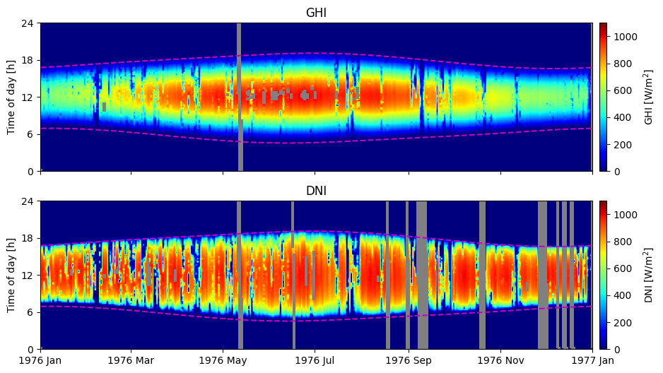
2D visualization as function of time and date#
One helpful plot to visualize the available data is a 2D plot of solar irradiance as a heat map as a function of time of day vs. day of the year.
Notice how especially the DNI is higher near the sunset times than the sunrise times. This significes that the timestamp refers to the past 15 minutes.
Show code cell source
# 2D plot of GHI & DNI where y-axis is hours and x-axis is day
df_2d = df[['ghi','dni']].set_index([df.index.date, df.index.hour*60+df_barstow.index.minute]).unstack(level=0)
df_2d = df_2d.reindex(np.arange(0, 1440,15)) # ensure all minutes are present
df_2d.index = df_2d.index/60 # necessary to first convert afterwards, due to rounding issues.

# Calculate sunrise times
days = pd.date_range(df.index[0], df.index[-1], tz=barstow.tz) # List of days for which to calculate sunrise/sunset
sunrise_sunset = barstow.get_sun_rise_set_transit(days, method='spa')

# Convert sunrise/sunset from Datetime to hours (decimal)
sunrise_sunset['sunrise'] = sunrise_sunset['sunrise'].dt.hour + sunrise_sunset['sunrise'].dt.minute/60
sunrise_sunset['sunset'] = sunrise_sunset['sunset'].dt.hour + sunrise_sunset['sunset'].dt.minute/60

# Calculate the extents of the 2D plot, in the format [x_start, x_end, y_start, y_end]
xlims = mdates.date2num([df_barstow.index[0].date(), df_barstow.index[-1].date()])
extent = [xlims[0], xlims[1], 0, 24]

fig, axes = plt.subplots(nrows=2, figsize=(12,6), sharex=True)
for ax, component in zip(axes, ['ghi','dni']): # names of plot
    im = ax.imshow(df_2d[component], aspect='auto', origin='lower', cmap='jet',
                   extent=extent, vmin=0, vmax=1100)
    ax.set_title(component.upper())
    ax.set_xlim(xlims)
    ax.set_yticks(np.arange(0,25,6))
    ax.set_ylabel('Time of day [h]')
    ax.set_facecolor('grey')
    ax.xaxis_date()
    ax.xaxis.set_major_formatter(mdates.DateFormatter('%Y %b'))
    ax.plot(mdates.date2num(sunrise_sunset.index), sunrise_sunset[['sunrise', 'sunset']], 'm--')
    cbar1 = fig.colorbar(im, ax=ax, orientation='vertical', pad=0.01, label=f"{component.upper()} [W/m$^2$]")
Visualization as function of solar elevation and zenith angle#
In order to detect possible shading from nearby objects and hills, it is useful to visualize the maximum irradiance as a function of solar elevation and zenith angle. Particularly the DNI plot is helpful in identifiying the local obstruction free horizon line.
Due to the 15-minute resolution a 2-degree resolution is used.
Show code cell source
df_2d = df.loc[df['apparent_elevation']>=0, ['ghi','dni']].groupby([df['azimuth'].divide(2).round(0).multiply(2), df['apparent_elevation'].divide(2).round(0).multiply(2)]).max().unstack(level=0).sort_index()

fig, axes = plt.subplots(nrows=2, figsize=(12,6), sharex=True)
for ax, component in zip(axes, ['ghi','dni']):
    extent = [df_2d[component].columns.min(), df_2d[component].columns.max(), df_2d[component].index.min(), df_2d[component].index.max()]
    im = ax.imshow(df_2d.loc[0:, component], aspect='auto', origin='lower', cmap='jet',
                        extent=extent, vmin=0, vmax=df_barstow[component].quantile(0.99))
    ax.grid(alpha=0.5)
    ax.set_xlim(0,360)
    ax.set_xticks(np.arange(0,360+60,60))
    ax.set_yticks(np.arange(0,round(df_2d.index.max()/10)*10+10+10,10))
    ax.set_ylim(0,None)
    ax.set_ylabel('Solar elevation [°]')
    cbar3 = fig.colorbar(im, ax=ax, pad=0.01, orientation='vertical', label='Max. {} [W/m$^2$]'.format(component))
axes[-1].set_xlabel('Solar azimuth [°E of N]')
axes[0].set_title('Maximum irradiance as a function of solar elevation and azimuth')
Text(0.5, 1.0, 'Maximum irradiance as a function of solar elevation and azimuth')
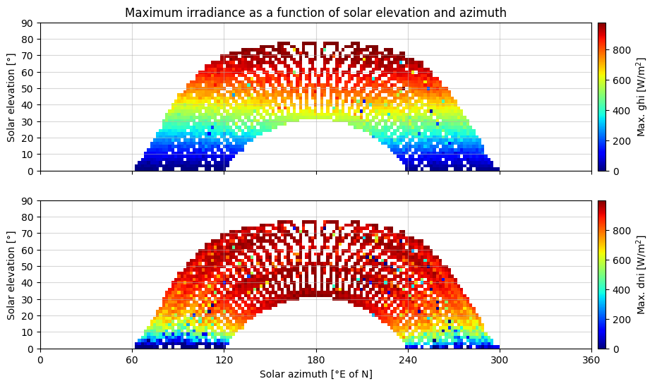
Based on the plots above, it seems that the local shading is limited to below 10° solar elevation.
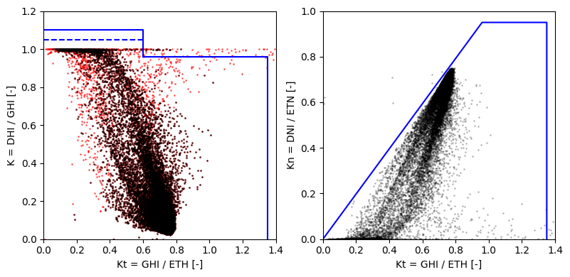
Quality-check plots#
The below plots visualize the normalize irradiance values. The blue lines represents the quality-control limits recommend by the BSRN.
Show code cell source
fig, axes = plt.subplots(ncols=2, figsize=(8,4))
df.plot.scatter(ax=axes[0], x='Kt', y='K', s=1, c='r', alpha=0.5)
df[df['ghi']>50].plot.scatter(ax=axes[0], x='Kt', y='K', s=1, c='k', alpha=0.5)

axes[0].set_xlim(0, 1.4), axes[0].set_ylim(0, 1.2)
axes[0].plot([0,0.6,0.6,1.35,1.35], [1.1,1.1,0.96,0.96,0], c='blue', label='limits')
axes[0].plot([0,0.6], [1.05,1.05], c='blue', linestyle='dashed', label='limits')
axes[0].set_xlabel('Kt = GHI / ETH [-]'), axes[0].set_ylabel('K = DHI / GHI [-]')


df.plot.scatter(ax=axes[1], x='Kt', y='Kn', s=1, c='k', alpha=0.2)
axes[1].set_xlim(0, 1.4), axes[1].set_ylim(0, 1)
axes[1].plot([0,0.96,1.35,1.35], [0,0.95,0.95,0], c='blue', label='limits')
axes[1].set_xlabel('Kt = GHI / ETH [-]'), axes[1].set_ylabel('Kn = DNI / ETN [-]')

plt.tight_layout()
Percentage of missing data#
It is also interesting to get a quantitative measure for the amount of missing data:
df.loc[df['apparent_elevation']>0, ['ghi','dni']].isna().mean().multiply(100).round(1).astype(str).add(' %')
ghi    0.9 %
dni    7.2 %
dtype: object
Clearly, the DNI measurements are errornous to a much higher degree than the GHI measurements. This is partly due to the fact that it is much easier to detect a faulty DNI measurement, but also that DNI sensors are much more prone to soiling and affected by tracker errors and misalignment.